Sudoku Solver Algorithm - Understanding the Logic

A Sudoku solver algorithm combines two ideas: constraint propagation, which repeatedly places every digit that is logically forced, and backtracking, which tries a candidate in the most constrained cell and undoes the choice if it leads to a contradiction. With the minimum-remaining-values heuristic guiding the search, this solves any valid 9×9 grid in milliseconds, including the puzzles designed to defeat naive solvers.
This article explains how the algorithm works, why the naive version is hopelessly slow, what each optimisation buys you, and how to write one yourself in Python. Our own free Sudoku solver uses exactly this approach.
The problem, stated precisely
Sudoku is a constraint satisfaction problem. You have 81 variables (the cells), each with a domain of 1 to 9, and a set of constraints: no two cells in the same row, column or 3×3 box may hold the same value. Some variables are pre-assigned — the givens.
Every cell has exactly 20 peers: 8 in its row, 8 in its column, and 4 more in its box that are not already counted. A digit placed in a cell is immediately excluded from all 20.
Formally, Sudoku generalised to n×n is NP-complete. In practice the 9×9 case is tiny, and a well-written solver finishes before you lift your finger from the key.
Why brute force fails
The naive algorithm tries every digit in every empty cell and checks validity at the end. With around 50 empty cells that is 950 combinations — roughly 5×1047. No computer will ever finish that.
Adding validity checks during the search rather than at the end cuts it enormously, because most branches die immediately. That single change turns an impossible problem into an easy one, and it is the whole idea behind backtracking.
Step one: constraint propagation
Before searching at all, the solver maintains a candidate set for every empty cell — the digits still allowed there. Two rules then fire repeatedly:
- Naked single. If a cell's candidate set shrinks to one digit, that digit is placed, and it is removed from the candidate sets of all 20 peers.
- Hidden single. If a digit has only one possible cell within a unit, it is placed there, even if that cell had other candidates.
Each placement triggers more eliminations, which may create more singles — a cascade. On easy and medium grids the cascade finishes the puzzle with zero searching. That is the single most important optimisation in any Sudoku solver.
Step two: backtracking
When propagation stalls, the solver must guess. The classic recursive shape:
- Find the empty cell with the fewest remaining candidates.
- If any empty cell has zero candidates, this branch is dead — return failure immediately.
- Try each candidate of the chosen cell in turn: place it, propagate, and recurse.
- If the recursion succeeds, the puzzle is solved. If it fails, undo the placement and try the next candidate.
- If every candidate fails, return failure to the caller.
Because the algorithm is complete, it finds the solution whenever one exists, and proves there is none when there is not.
Why minimum remaining values matters so much
Choosing which cell to branch on is the difference between milliseconds and minutes.
Picking cells in reading order means often branching on a cell with 6 or 7 candidates — a wide, shallow tree with enormous fan-out. Picking the cell with the fewest candidates — the MRV heuristic, sometimes called "fail first" — means usually branching on a cell with 2 candidates, halving the tree at each level and discovering contradictions almost immediately.
| Strategy | Typical hard grid |
|---|---|
| Pure brute force, check at end | Never finishes |
| Backtracking, cells in order | Thousands to millions of steps |
| Backtracking + propagation | Hundreds of steps |
| Propagation + MRV | Tens of steps, sub-millisecond |
A working Python solver
Roughly forty lines, using a dictionary of candidate strings. The grid is given as an 81-character string with 0 or . for blanks.
That structure — assign, propagate, recurse on the most constrained cell — is the whole solver. Everything else is optimisation.
Writing the solver: the code in detail
Representing the grid
The cleanest representation is a dictionary mapping each of the 81 cell names to a string of its remaining candidates. A solved cell holds a one-character string; an untouched cell holds "123456789". This makes elimination a string operation and makes "is it solved?" a length check, with no separate bookkeeping.
The eliminate function
Everything happens here. Removing a candidate d from cell c triggers two consequences. First, if c now has one candidate left, that value must be eliminated from all 20 peers — recursively. Second, for each unit containing c, if d now has only one possible cell in that unit, assign it there. If any cell reaches zero candidates, return failure and let the caller backtrack.
The search function
If every cell has exactly one candidate, return the grid. Otherwise select the unsolved cell with the fewest candidates and try each one: copy the dictionary, assign, recurse. Copying is what makes undo free — you never mutate the parent state, so failure just discards the copy.
Optimisations that actually matter
| Optimisation | Effect |
|---|---|
| Constraint propagation | Largest single win; easy grids need no search at all |
| MRV cell selection | Cuts branching factor from ~6 to ~2 |
| Precomputed peer table | Removes index arithmetic from the hot loop |
| Bitmask candidates | Elimination becomes a single AND; 5–10× faster |
| In-place undo | Avoids copying state at every node |
| Hidden-single detection | Roughly halves the search on medium grids |
The first two are worth more than everything below them combined. A clean propagation-plus-MRV solver in a slow language beats a heavily optimised brute-force solver in a fast one.
Testing a solver you have written
- Verify correctness, not just completion. Check the output against all three constraints rather than trusting the search. An off-by-one in the peer table produces plausible-looking wrong grids.
- Test the empty grid. It must return a valid complete grid. This exercises the search path with no propagation help.
- Test an invalid grid. Two identical digits in one row must return failure, not loop forever.
- Test a multi-solution grid. Remove clues until several solutions exist; a counting variant should report more than one.
- Test the known hard cases. Grids designed to defeat solvers, such as Arto Inkala's, should still finish in milliseconds. If they take seconds, your MRV is not working.
- Time a batch. A thousand mixed puzzles should complete in a second or two. A per-puzzle average above a millisecond means something is wrong.
Common bugs
- Forgetting the box constraint. The solver appears to work and produces grids that fail box validation. Always test all three units.
- Mutating shared state. If the recursion modifies the parent's candidate structure, backtracking corrupts the grid. Copy, or implement a proper undo stack.
- Missing hidden singles. The solver still works but is far slower, because it searches where it could have deduced.
- Infinite recursion on invalid input. Always check for zero-candidate cells before recursing.
- Assuming uniqueness. A generator that skips the solution-count check produces broken puzzles that no logic can resolve.
Other approaches
Dancing Links (Algorithm X)
Sudoku can be reformulated as an exact cover problem: choose a set of rows from a 729×324 binary matrix so that every column is covered exactly once. Donald Knuth's Algorithm X with the Dancing Links data structure solves it very fast and is the classic academic approach. It is elegant but harder to write and rarely faster in practice than propagation plus MRV on 9×9 grids.
SAT solvers
Encode the constraints as boolean clauses and hand them to an off-the-shelf SAT solver. Trivial to implement and extremely fast, but the encoding step dominates the runtime for a single puzzle.
Stochastic methods
Simulated annealing and genetic algorithms can solve Sudoku but are strictly worse than the logical approach: slower, non-deterministic, and unable to prove that no solution exists.
Generating puzzles, and checking uniqueness
The solver is also the generator. To create a puzzle:
- Produce a complete valid grid by running the solver on an empty board with randomised candidate order.
- Remove a given digit at random.
- Run a solver that counts solutions and stops at two. If the count is still exactly one, keep the removal; otherwise put the digit back.
- Repeat until no further digit can be removed without losing uniqueness.
The uniqueness check in step 3 is what separates a real puzzle from a broken one. Free apps that skip it produce grids with multiple solutions — which is why some app puzzles feel impossible in a way that no logic can resolve.
Rating difficulty programmatically
Difficulty is not clue count. Generators rate a grid by running a solver that applies human techniques in ascending order of complexity and recording the hardest one required.
| Rating | Hardest technique needed |
|---|---|
| Easy | Hidden singles |
| Medium | Naked and hidden pairs |
| Hard | Pointing pairs, box-line reduction |
| Expert | X-Wing, Swordfish, XY-Wing, chains |
This is why a 26-clue grid can be far harder than a 24-clue one, and why ratings are not comparable between publishers.
Performance in practice
- An easy grid finishes on propagation alone, with no search at all.
- A hard grid typically needs a few dozen backtracking steps.
- Grids built specifically to defeat solvers — such as Arto Inkala's designs — may need thousands of steps, which is still a few milliseconds.
- The 17-clue minimum was proven in 2012 by exhaustively checking all possible 16-clue configurations, a computation of about 7 million CPU hours.
Frequently asked questions
How does a Sudoku solver algorithm work?
It combines constraint propagation with backtracking. It tracks the remaining candidates for every cell, places every forced digit, and when it stalls it branches on the cell with the fewest candidates, undoing the choice if a contradiction appears.
What algorithm is best for solving Sudoku?
Constraint propagation plus backtracking with the minimum-remaining-values heuristic. It is simple to write and solves any 9×9 grid in milliseconds. Dancing Links and SAT solvers work too but are not faster in practice at this size.
What is backtracking in a Sudoku solver?
Placing a candidate in a cell, continuing the search, and undoing that placement if it leads to a contradiction. Combined with propagation it explores only a tiny fraction of the possible grids.
What is constraint propagation?
Repeatedly applying two rules: a cell with one remaining candidate gets that digit, and a digit with one possible cell in a unit is placed there. Each placement removes candidates from 20 peers, which often cascades.
What is the minimum remaining values heuristic?
Always branching on the unsolved cell with the fewest candidates. It keeps the search tree narrow and surfaces contradictions early, and it is the difference between milliseconds and minutes.
How many peers does a Sudoku cell have?
Twenty: eight in its row, eight in its column, and four more in its 3×3 box that are not already counted. Placing a digit removes it from all twenty candidate sets.
Why is brute force too slow for Sudoku?
With about 50 empty cells there are roughly 9^50 combinations if you only check validity at the end. Checking constraints during the search kills most branches immediately, which makes the problem easy.
Is Sudoku NP-complete?
Generalised n×n Sudoku is NP-complete. The standard 9×9 case is small enough that a good solver finishes in microseconds, so the theoretical result has no practical impact.
What is Dancing Links?
Knuth's implementation of Algorithm X for exact cover problems. Sudoku maps onto a 729×324 cover matrix. It is elegant and fast, though rarely faster than propagation with MRV on 9×9 grids.
How do you generate a Sudoku puzzle?
Solve an empty grid with randomised ordering to get a full solution, then remove digits one at a time, keeping each removal only if a solution-counting solver still finds exactly one solution.
How does a program rate Sudoku difficulty?
By running a solver that applies human techniques in ascending complexity and recording the hardest one needed. Clue count is a poor predictor; the required technique is what defines difficulty.
Can a solver detect an invalid puzzle?
Yes. Because the algorithm is complete, exhausting the search without success proves no solution exists. A counting variant also detects puzzles with multiple solutions, which means the grid is faulty.
How fast is a good Sudoku solver?
Easy grids finish on propagation alone with no search. Hard grids take a few dozen backtracking steps. Even puzzles built to defeat solvers finish in a few milliseconds.
Try it
Enter any grid into our free Sudoku solver to see constraint propagation and MRV backtracking in action — complete solution, in under a second.
Next, read: How to Solve Sudoku — The Complete Guide · Free Sudoku Solver · How to Solve Hard Sudoku